Bivariate quantiles

library(tidyverse)
library(qpd)
library(hrbrthemes)

Introduction

One of the recent papers I included in Quantile Statistics Overlay is Nair and Vineshkumar (2023). Prof. N. Unnikrishnan Nair is the former head of Statistics Department at the Cochin University of Science and Technology (Kerala, India). His co-author here is Dr B. Vineshkumar, the Assistant Professor of Statistics at the Government Arts College, Thiruvananthapuram (also in Kerala). Prof. N.U. Nair and Dr. Vineshkumar have been prolific contributors to the field of quantile statistics and I will be including more of their work into our overlay publication.

Bivariate Quantiles

The earlier paper Vineshkumar and Nair (2019) provided the helpful definition of bivariate quantiles, which extends the univariate case for quantile function of \(X\)

\[ \begin{gathered} Q_i(u_i)=\inf\{x_i\vert F_i(x_i)\geq u_i\}, \; u_i\in I=[0,1] \end{gathered} \]

The bivariate quantile function of \((X_1,X_2)\) is then given by

\[ Q(u_1, u_2)=(Q_1(u_1),Q_{21}(u_2\vert u_1))\\ \]

where

\[ \begin{gathered} Q_1(u_1)=\inf\{x_1\vert F_1(x_1)\geq u_1\}\\ Q_{21}(u_2\vert u_1)=\inf\{x_2\vert P(X_2\leq x_2 \vert X_1>Q_1(u_1))\geq u_2\} \end{gathered} \]

Recall, that the the joint survival function is \(\bar{F}(x_1,x_2)=1-F_1(x_1)-F_2(x_2)+F(x_1,x_2)\) (Kundu and Gupta 2009), which is a multivariate extension of the univariate survival function \(\bar{F}(x)=1-F(x)\). The authors factorize the joint survival function \(\bar{F}(x_1,x_2)\) as follows:

\[ \bar{F}(x_1, x_2)=P(X_1> x_1)P(X_2> x_2 \vert X_1 > x_1)= \bar{F}(x_1)\bar{F}_{21}(x_1,x_2) \]

The conditional distribution function \(F_{21}(x_1,x_2)\) should not be confused with the marginal distribution function \(F_2(x_2)\). The conditional distribution function can be computed from the joint distribution function using the formulae above (with the help of the marginal).

The conditional survival function \(\bar{F}_{21}(x_1,x_2)\) and the corresponding conditional quantile function \(Q_{21}(u_2\vert u_1)\) constitute the main element in the definition of bivariate quantiles.

\[ Q_{21}(u_2\vert u_1)=\inf\{x_2\vert F_{21}(Q_1,x_2)\geq u_2\} \]

We can find the conditional quantile function \(Q_{21}\) by inverting the conditional distribution function \(F_{21}\) for \(x_2\), and substituting the marginal \(Q_1(u_1)\) instead of \(x_1\).

Examples

Nair and Vineshkumar (2023) provide several examples which might be illuminating to have a closer look at.

Mardia’s bivariate Pareto distribution

The authors provide a survival function for the Mardia’s bivariate Pareto distribution¹

\[ \bar{F}(x_1, x_2)=(x_1+x_2+1)^{-c}, \; x_1, x_2>1, c>0 \]

The marginal quantile functions \(Q_i(u_i)=(1-u_i)^{-1/c}-1\), therefore the marginal distribution functions are \(F_i(x_i)=-\left(x_i+1\right)^{-c}+1\) for \(i=1,2\). We can find the conditional survival function \(\bar{F}_{21}(x_1,x_2)=P(X_2>x_2\vert X_1>x_1)\), and corresponding conditional distribution function \(F_{21}(x_1,x_2)\) as

\[ \begin{gathered} \bar{F}_{21}(x_1,x_2)=\frac{\bar{F}(x_1, x_2)}{\bar{F}_1(x_1)}=\frac{(x_1+x_2+1)^{-c}}{(x_1+1)^{-c}}\\ F_{21}(x_1,x_2)=1-\left(\frac{x_1+x_2+1}{x_1+1}\right)^{-c} \end{gathered} \]

Now, we need to invert this, i.e. solve it for \(x_2\), because we are interested in conditional quantile function \(Q_{21}(u2\vert u1)\).

\[ \begin{gathered} u_2=1-\left(\frac{x_1+x_2+1}{x_1+1}\right)^{-c}\\ (1-u_2)^{-1/c}=\frac{x_1+x_2+1}{x_1+1}\\ (1-u_2)^{-1/c}(x_1+1)=x_1+x_2+1\\ (1-u_2)^{-1/c}(x_1+1)-x_1-1=x_2 \end{gathered} \]

We are almost there. Now we drop in marginal \(Q_1(u_1)=(1-u_1)^{-1/c}-1\) instead of \(x_1\).

\[ \begin{gathered} (1-u_2)^{-1/c}([(1-u_1)^{-1/c}-1]+1)-[(1-u_1)^{-1/c}-1]-1=x_2\\ (1-u_2)^{-1/c}(1-u_1)^{-1/c}-(1-u_1)^{-1/c}=x_2\\ Q_{21}(u_1, u_2)=(1-u_1)^{-1/c}[(1-u_2)^{-1/c}-1] \end{gathered} \]

Which is exactly the solution provided in the paper. Now we can proceed to sampling from our brand new bivariate quantile function.

qmardiapareto1 <- function(u, cc){
  mic <- (-1/cc) #minus inverse c
  (1-u)^mic-1
}

qmardiapareto21 <- function(u2, u1, cc){
  mic <- (-1/cc)
  (1-u1)^mic*((1-u2)^mic-1)
}

set.seed(1)
n <- 1e3
cc <- 10
tibble::tibble(u1=runif(n),
               u2=runif(n),
               x1=qmardiapareto1(u1,cc),
               x2=qmardiapareto21(u2, u1, cc)) %>%  
  ggplot()+
  geom_point(aes(x1, x2))+
  theme_ipsum_rc(grid_col="grey95")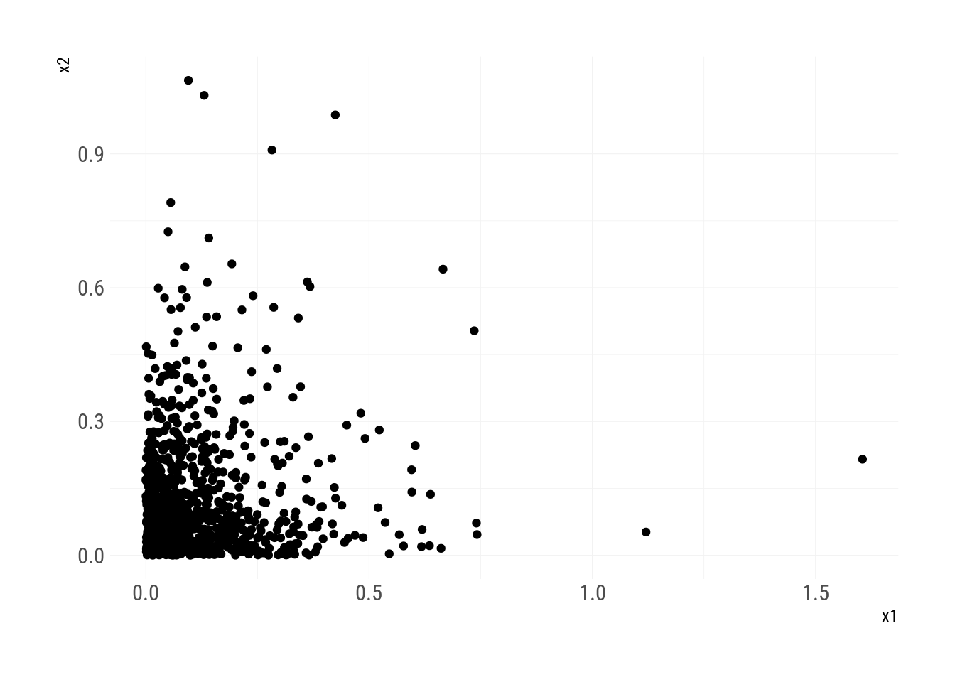

Bivariate Pareto distribution

Another variant of bivariate Pareto distribution is provided in Vineshkumar and Nair (2019). Here, the joint survival function is given by

\[ \bar{F}(x_1, x_2)=(1+a_1x_1+a_2x_2+bx_1x_2)^{-p} \]

where \(x_1,x_2>0, \;a_1,a_2>0, \; 0\leq b \leq (p-1)a_1a_2\). The marginal distribution is given by \(F_i(x_i)=1-(1+a_ix_i)^{-p}\) and the inverse is \(Q_i(u_i)=\frac{1}{a_i}[(1-u_i)^{-1/p}-1]\)².

We find the conditional survival and distribution functions as

\[ \begin{gathered} \bar{F}_{21}(x_1,x_2)=\frac{\bar{F}(x_1, x_2)}{\bar{F}_1(x_1)}=\frac{(1+a_1x_1+a_2x_2+bx_1x_2)^{-p}}{(1+a_1x_1)^{-p}}\\ F_{21}(x_1,x_2)=1-\left(\frac{1+a_1x_1+a_2x_2+bx_1x_2}{1+a_1x_1}\right)^{-p} \end{gathered} \]

Now we invert \(F_{21}\) for \(x_2\).

\[ \begin{gathered} u_2=1-\left(\frac{1+a_1x_1+a_2x_2+bx_1x_2}{1+a_1x_1}\right)^{-p}\\ (1-u_2)^{-1/p}=\frac{1+a_1x_1+a_2x_2+bx_1x_2}{1+a_1x_1}\\ (1-u_2)^{-1/p}({1+a_1x_1})-1-a_1x_1=a_2x_2+bx_1x_2\\ (1-u_2)^{-1/p}({1+a_1x_1})-1-a_1x_1=x_2(a_2+bx_1)\\ x_2=\frac{\left(1-u_2\right)^{-\frac{1}{p}}+a_1x_1\left(1-u_2\right)^{-\frac{1}{p}}-a_1x_1-1}{a_2+bx_1} \end{gathered} \]

And drop in the marginal quantile function instead of \(x_1\).

\[ \begin{gathered} Q_{21}(u_2\vert u_1)=\frac{\left(1-u_2\right)^{-\frac{1}{p}}+a_1x_1\left(1-u_2\right)^{-\frac{1}{p}}-a_1x_1-1}{a_2+bx_1}\\ Q_{21}(u_2\vert u_1)=\frac{\left(1-u_2\right)^{-\frac{1}{p}}+a_1[\frac{1}{a_1}[(1-u_1)^{-1/p}-1]]\left(1-u_2\right)^{-\frac{1}{p}}-a_1[\frac{1}{a_1}[(1-u_1)^{-1/p}-1]]-1}{a_2+b[\frac{1}{a_1}[(1-u_1)^{-1/p}-1]]}\\ Q_{21}(u_2\vert u_1)=\frac{\left(1-u_2\right)^{-\frac{1}{p}}+[(1-u_1)^{-1/p}-1]\left(1-u_2\right)^{-\frac{1}{p}}-[(1-u_1)^{-1/p}-1]-1}{a_2+\frac{b}{a_1}[(1-u_1)^{-1/p}-1]}\\ Q_{21}(u_2\vert u_1)=\frac{a_1[\left(1-u_2\right)^{-\frac{1}{p}}(1-u_1)^{-1/p}-(1-u_1)^{-1/p}]}{a_1a_2+b[(1-u_1)^{-1/p}-1]}\\ Q_{21}(u_2\vert u_1)=\frac{a_1(1-u_1)^{-1/p}[\left(1-u_2\right)^{-\frac{1}{p}}-1]]}{a_1a_2+b[(1-u_1)^{-1/p}-1]} \end{gathered} \]

Which is exactly the result in the paper.

qotherpareto1 <- function(u, a, p){
  mip <- (-1/p) #minus inverse p
  1/a*(1-u)^mip-1
}

qotherpareto21 <- function(u2, u1, a2, a1, b, p){
  mip <- (-1/p)
  num <- a1*((1-u2)^mip-1)*((1-u1)^mip)
  den <- a1*a2+b*((1-u1)^mip-1)
  num/den
}

set.seed(1)
n <- 1e3
p <- 10
a2 <- 0.2; a1 <- 0.4; b <- 0.1
tibble::tibble(u1=runif(n),
               u2=runif(n),
               x1=qotherpareto1(u1, a1, p),
               x2=qotherpareto21(u2, u1, a2, a1, b, p)) %>%  
  ggplot()+
  geom_point(aes(x1, x2))+
  theme_ipsum_rc(grid_col="grey95")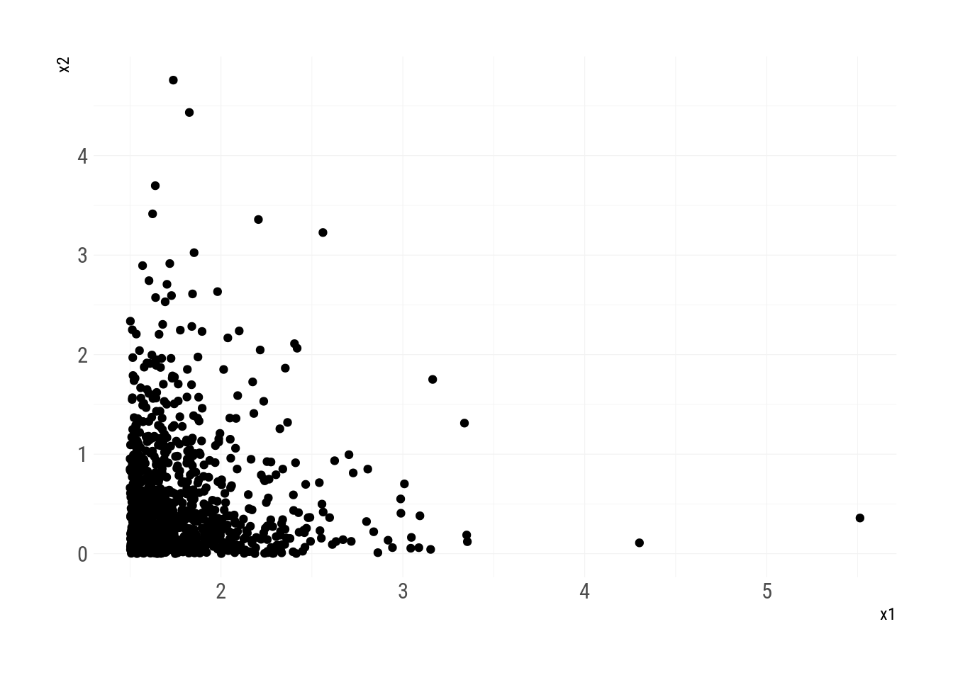

Gumbel’s bivariate exponential distribution

Gumbel (1960) proposed two kinds of bivariate exponential distributions. The Type I distribution has the survival function

\[ \bar{F}(x_1, x_2)=\exp[-\lambda_1x_1-\lambda_2x_2-\theta x_1x_2]\\ \]

The marginal quantile function is, of course, \(Q_i(u_i)=-\ln(1-u_i)/\lambda_i\) and the corresponding marginal distribution function is \(F_i(x_i)=1-\exp[-\lambda_i x_i]\).

Gumbel (1960) defined the distribution by the joint distribution function, which is slightly more verbose than the survival function.

\[ \begin{gathered} \bar{F}(x_1,x_2)=1-F_1(x_1)-F_2(x_2)+F(x_1,x_2)\\ F(x_1, x_2)=\exp[-\lambda_1x_1-\lambda_2x_2-\theta x_1x_2]-1+1-\exp[-\lambda_1 x_1]+1-\exp[-\lambda_2 x_2]\\ F(x_1, x_2)=1-\exp[-\lambda_1 x_1]-\exp[-\lambda_2 x_2]+\exp[-\lambda_1x_1-\lambda_2x_2-\theta x_1x_2] \end{gathered} \]

The first step is to find the conditional survival and distribution functions.

\[ \begin{gathered} \bar{F}_{21}(x_1,x_2)=\frac{\bar{F}(x_1, x_2)}{\bar{F}_1(x_1)}=\frac{\exp[-\lambda_1x_1-\lambda_2x_2-\theta x_1x_2]}{\exp[-\lambda_1 x_1]}\\ F_{21}(x_1,x_2)=1-\exp[-\lambda_2x_2-\theta x_1x_2] \end{gathered} \]

Now we need to invert this conditional distribution function for \(u_2\) and drop in the marginal quantile function \(Q_1(u_1)\) in place of \(x_1\).

\[ \begin{gathered} u_2=1-\exp[-\lambda_2x_2-\theta x_1x_2]\\ 1-u_2=\exp[-\lambda_2x_2-\theta x_1x_2]\\ \ln(1-u_2)=-\lambda_2x_2-\theta x_1x_2\\ \ln(1-u_2)=x_2(-\lambda_2-\theta x_1)\\ \frac{\ln(1-u_2)}{-\lambda_2-\theta x_1}=x_2\\ \frac{\ln(1-u_2)}{-\lambda_2-\theta [-\ln(1-u_1)/\lambda_1]}=x_2\\ \frac{\lambda_1\ln(1-u_2)}{-\lambda_2\lambda_1-\theta [-\ln(1-u_1)]}=x_2\\ Q_{21}(u_2\vert u_1)=\frac{-\lambda_1\ln(1-u_2)}{\lambda_2\lambda_1-\theta \ln(1-u_1)}\\ \end{gathered} \]

So the Gumbel bivariate exponential function becomes

\[ Q(u_1, u_2)=\left( \frac{1}{\lambda_1\ln(1-u_1)}, \frac{-\lambda_1\ln(1-u_2)}{\lambda_2\lambda_1-\theta \ln(1-u_1)}\right) \]

This is the exactly the result reported in the paper.

qgumbelexp1 <- function(u, lambda){
 -log(1-u)/lambda
}

qgumbelexp21 <- function(u2, u1, lambda2, lambda1, theta){
 -lambda1*log(1-u2)/(lambda1*lambda2-theta*log(1-u1))
}

set.seed(1)
n <- 1e3
theta <- 3
lambda1 <- 1; lambda2 <- 2
tibble::tibble(u1=runif(n),
               u2=runif(n),
               x1=qgumbelexp1(u1, lambda1),
               x2=qgumbelexp21(u2, u1, lambda2, lambda1, theta)) %>%  
  ggplot()+
  geom_point(aes(x1, x2))+
  theme_ipsum_rc(grid_col="grey95")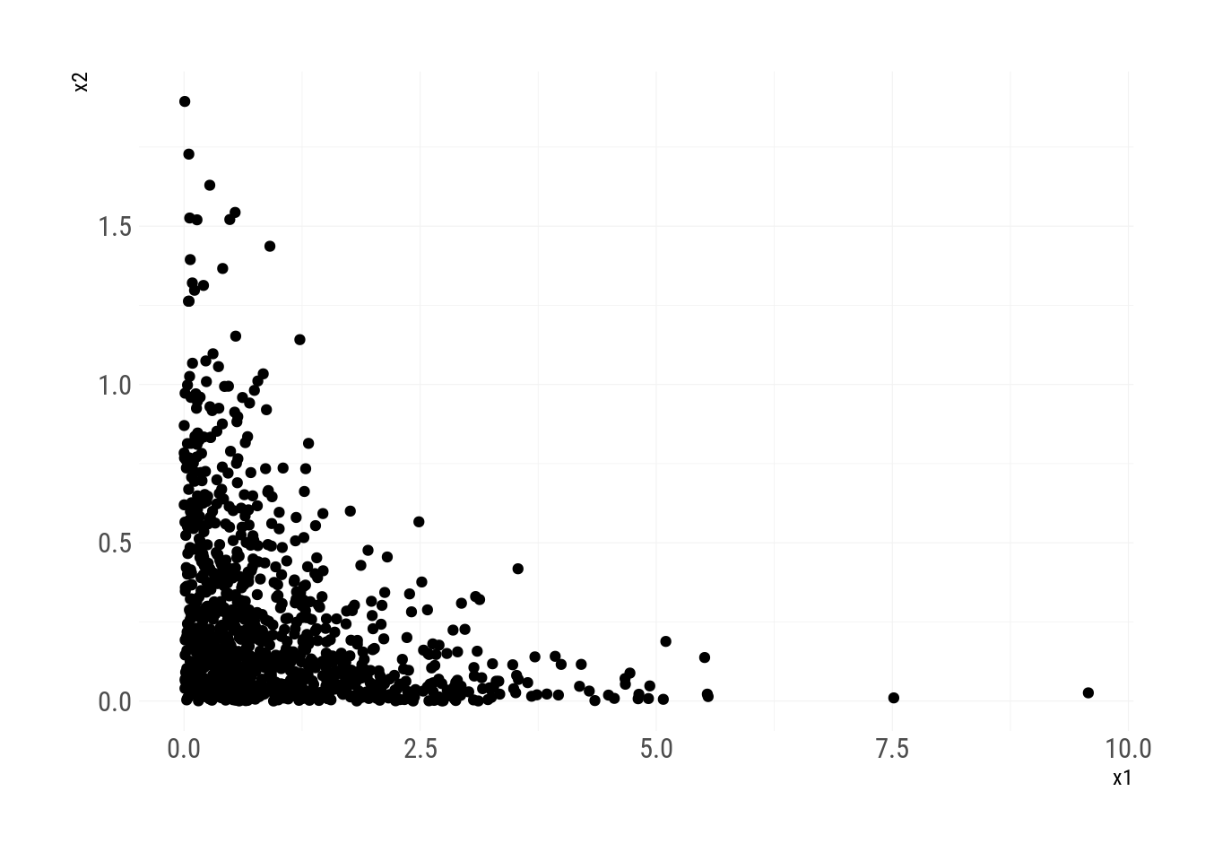

Properties of bivariate quantiles

You might ask: “Wow, that’s a lot of math! Why do we care about bivariate quantiles?” and “Well, don’t they require invertible joint distribution functions?”

The cool thing about bivariate quantile functions (bQFs) come from their properties discussed in Nair and Vineshkumar (2023). The authors list 9 properties, which are, in some sense, extensions of Gilchrist (2000) properties for univariate QFs. In particular, the properties 6 through 9 are pretty cool.

The authors start by stating that the conditional bQFs \(Q_{21}\) do not necessarily have to come from inverting the conditional distribution function \(F_{21}\). In fact, any left-continuous, increasing function in \(u_2\), for all \(u_1 \in [0,1]\) can be picked at \(Q_{21}\) (provided that the combination \((Q_1, Q_{21})\) results in a meaningful bivariate model).

It turns out (Property 6) that the conditional bQF \(Q_{21}(u_2\vert u_1)\) can be constructed as a sum of two univariate QFs, i.e. this represents a valid bQF \((Q_1(u_1), Q_1(u_1)+Q_2(u_2))\). If \(Q_1\) is left-bounded at zero, i.e. \(Q_1(0)=0\) then the marginals of such bQF are \(Q_1(u_1)\) and \(Q_2(u_2)\)! This finding generalizes Gilchrist’s “addition rule” (Gilchrist 2000). Similar to the univariate case, also works for quantile densities (Property 7).

Property 8 says that for the positive QFs the product is also a valid conditional bQF, generalizing the “product rule” (Gilchrist 2000). Finally, Property 9 generalizes the “Q-transformation rule”, postulating that for every increasing transformation functions \(T_1\) and \(T_2\), \(\left[T_1(Q_1(u_1)), T_1(Q_1(u_1))+T_2(Q_2(u_2))\right]\) is also a valid bQF. The main implication here is that the bQFs can be defined without the reference to the join distribution function (and even without closed form \(F(x_1, x_2)\))!

Conclusion

So why do we care? Given what we have discussed in Perepolkin, Goodrich, and Sahlin (2021), priors can be defined using the quantile functions without the reference to the densities. This not only means that you don’t need PDFs to define the prior, but also that you don’t need QDF, because it will cancel itself with the Jacobian.

Now with bQFs, you can define the bivariate priors using quantile functions, provided that the conditional bQF \(Q_{21}\) that you crafted makes sense.

Perhaps some Stan examples would be in order. I am sure we will come back to the bivariate quantiles for some cool quantile distribution application soon.

References

Gilchrist, Warren. 2000. Statistical Modelling with Quantile Functions. Boca Raton: Chapman & Hall/CRC.

Gumbel, E. J. 1960. “Bivariate Exponential Distributions.” Journal of the American Statistical Association 55 (292): 698–707. https://doi.org/10.2307/2281591.

Kundu, Debasis, and Rameshwar D. Gupta. 2009. “Bivariate Generalized Exponential Distribution.” Journal of Multivariate Analysis 100 (4): 581–93. https://doi.org/10.1016/j.jmva.2008.06.012.

Nair, N. Unnikrishnan, and B. Vineshkumar. 2023. “Properties of Bivariate Distributions Represented Through Quantile Functions.” American Journal of Mathematical and Management Sciences 0 (0): 1–12. https://doi.org/10.1080/01966324.2021.2016522.

Perepolkin, Dmytro, Benjamin Goodrich, and Ullrika Sahlin. 2021. “The Tenets of Quantile-Based Inference in Bayesian Models.” Preprint. https://osf.io/enzgs: Open Science Framework. https://doi.org/10.31219/osf.io/enzgs.

Vineshkumar, Balakrishnapillai, and Narayanan Unnikrishnan Nair. 2019. “Bivariate Quantile Functions and Their Applications to Reliability Modelling.” Statistica 79 (1, 1): 3–21. https://doi.org/gpdd87.

Footnotes

1. There seems to be a typo in the paper. It says -1 instead of +1 in the survival function

2. Note that the paper missed the square brackets around the basic quantile function

Citation

BibTeX citation:

@online{perepolkin2023,
  author = {Dmytro Perepolkin},
  title = {Bivariate Quantiles},
  date = {2023-02-28},
  url = {https://www.ddrive.no/posts/2023-02-28-bivariate-quantiles/},
  langid = {en}
}

For attribution, please cite this work as:

Dmytro Perepolkin. 2023. “Bivariate Quantiles.” $D /Drive Blog. February 28, 2023. https://www.ddrive.no/posts/2023-02-28-bivariate-quantiles/.